Week 8b: AOD Sweeping and CuPy Acceleration

Alex

This week I was able to successfully utilize the controller software for its sweeping function. While changing parameters, I found that scanning outside of the range from 100-200MHz started to produce distorted waveforms. Brimrose helped inform me that some distortion may be present in the output waveform due to the presence of harmonics. We added a frequency analysis measurement to the oscilloscope to follow its steps in increasing frequency to the maximum and then its reset.

If we were to test the device and its sweeping function using a spectrum analyzer, it would take the form of a moving spike.

After this was accomplished, I attempted to input the 1560nm laser to the Bragg cell of the AOD in order to observe both the deflected angle and the input via an Infrared card. I first passed an Infrared laser through the unit to make sure the height and angle were aligned. I then switched the input to the Menlo Systems laser and placed the IR card on the output, close to the cell. I then rotated the card around to identify the point at which the laser could be observed via a red dot.

While a red dot was observed, I could not find the deflected point even with varying frequencies in the specified range. I plan to reread the setup and realign the laser through the cell in order to hopefully gain better results. I have followed up again with Brimrose for assistance in this matter.

Looking ahead, the AOD has a specified deflection angle of 30mrad which equates to 1.79 degrees. This means that at its deflection angle, it will oscillate at that point +/- 1.79 degrees. Through some preliminary calculations, it was determined that the arclength necessary will be 16cm. We are now in the early design stages in order to implement this into the system. The first two options that come to mind are a horizontal design of 16cm or to utilize mirrors to make a more compact version. This will be discussed at length with the team.

Trevor

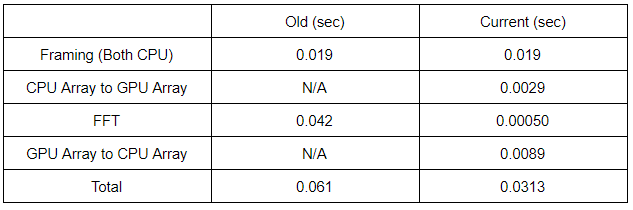
This week I looked into what parts of the processing code took the most amount of time to run. It turns out that the framing portion of the program takes up more than 90% of the processing time, while the FFT is the remaining 10% or so. So far I was only able to get the FFT running on the GPU. I tried to rewrite portions of the framing code to be compatible with CuPy, so far the there are errors in mismatching data structures. NumPy’s arrays are distinct from CuPy arrays, thus certain functions used in the framing function are incompatible with CuPy arrays. I will be working on altering the framing function in the coming days.

In terms of visualization, VisPy is still being looked into. In addition to VisPy, Visbrain is another option I am looking at. More research will need to be done on this aspect.

For improving the framerate, several options have been brought up. Due to the insufficient amount of data points needed for the GPU to accelerate the program, a proposed solution to combine multiple queues into one. For example, rather than processing a queue of 2 million points, the idea is to process a queue of 10 million points, effectively combing 5 queues into one for processing. In addition to that, one the hardware side, we will be switching to the Tektronix MS054 oscilloscope. We have stated before that is oscilloscope was unviable because of the lack of bandwidth to capture the entire signal, but this is only for the dual probe system. Our project will be reverting back to the single probe form factor which the MS054 can capture. While the MS054 does not have the capability to stream data like with the previously used DSA 72004C, its single-shot capture is quick enough that the time lost is minimal. The biggest reason for the switch is to be able to utilize the USB 3.0 ports available on the MS054 which would greatly increase the ceiling for our framerate from 6 FPS to approximately 312 FPS, assuming a 2MB frame size. This are all the improvements that can be done without the AOD. However, once the AOD is working and implemented, the improvements will be even greater

Finally, I ran the same FFT speed test as last week using my personal computer. This was to test if the performance of NumPy and CuPy was similar on different systems. The graph for this test is shown in Figure 1.

Figure 1: NumPy vs CuPy FFT

It can be seen in the graph that at approximately 2.4 million data points the GPU overtakes the CPU in speed. While the overall linear nature of the two FFT methods remain fairly consistent, the point in which the GPU performs faster is nearly half of that in the lab, being 4.6 million. This could be contributed to the more powerful CPU used in the lab if it weren’t for one glaring discrepancy. My objectively inferior PC outperformed the PC in the lab on both the CPU and GPU tests, more so on the GPU. My theory is that because the lab’s computer is generally always powered on, and is always having background tasks eating up ram that the performance takes a hit. Opposing that, with my PC, I ran my tests with a very slight amount of background tasks. This is the most viable theory I have, as my i7-7700k and GTX 1070 should not be able to outperform a Ryzen 9 3900x and GTX 2080 SUPER under similar circumstances. While an anomaly, this wasn’t the main point of the tests. I was able to see that across two different systems the improvements of the GPU over the CPU are prominent past a certain point.